FAFS Part 2: Building Blocks

In this part, we’ll explore the CUDA operations that form the foundation of our Flash Attention kernel. Flash Attention’s performance depends on two factors: maximizing compute throughput through tensor cores and minimizing memory bottlenecks through efficient data movement.

To understand why these factors matter, consider the arithmetic complexity of a typical attention slice: 64 query vectors attending to 4,096 key+value vectors, with . For the attention formula,

the operation count is approximately 68.4M floating-point operations, while we only need to load about 2.1M bytes from GMEM. This gives us an arithmetic intensity of ~32, meaning we perform 32 mathematical operations per byte loaded from memory. You can find code for calculating the arithmetic intensity in the appendix.

This high arithmetic intensity makes Flash Attention perfect for tensor cores. These specialized compute units deliver significantly higher throughput than regular floating point units, but they achieve peak performance when computation heavily outweighs memory access. Our 32:1 ratio means the tensor cores can stay busy performing matrix operations while memory transfers happen in the background.

We’ll build our toolkit of instructions in 3 stages, using the most performant instructions on Ampere in each:

1. High-throughput matrix operations: The mma (matrix multiply-accumulate) instruction for tensor core utilization
2. Efficient memory operations: Data movement primitives that maintain high bandwidth utilization
3. Supporting operations: Data type conversions and other essential details

Matrix Multiplication

Flash Attention’s performance hinges on two matrix multiplications, so let’s see how we can use Ampere’s tensor cores to accelerate these operations. For our kernels, the inputs and outputs will be bf16/fp16 tensors and we’ll calculate softmax in fp32 for numerical stability.

Tensor cores on Ampere work with fragments, which are matrix tiles stored in thread registers.

Fragment Definition

Throughout this series, we’ll use the term fragment to specifically refer to an tile stored in the register file across a warp, where each thread in the warp holds just 2 elements, but the entire warp collaborates to perform the multiplication. This is the fundamental unit of tensor core operations.

The mma Instruction

So how do we actually program these tensor cores? That’s where the mma (matrix multiply-accumulate) ptx instruction comes in. There is another instruction on to program tensor cores: wmma, but we’ll use mma because the fragment layout is transparent. For those more curious about the thought process behind this choice, you can check out wmma API.

The operation that mma performs is D = AB^T + C, where:

• A has shape (m, k)
• B has shape (n, k)
• C and D have shape (m, n) and can point to the same location in memory

Even though we store B in row major format (elements in the same row are next to each other in memory), the mma operation multiplies the transpose of B. This is important to keep in mind when we map our attention tensors to these operands.

The operands have the corresponding shapes and dtypes for the specific mma instruction we’ll be using, which has dimensions (m = 16, n = 8, k = 16). There are two instructions available for 16-bit inputs with 32-bit accumulation on Ampere: m16n8k8 and m16n8k16. We’ll pick m16n8k16 because it’s slightly more efficient.

Operand	DType	Shape (Variables)	Shape (Elements)	Shape (Fragments)	Shape (Registers)
A	BF16/FP16	(m, k)	(16, 16)	(2, 2)	(2, 2)
B	BF16/FP16	(n, k)	(8, 16)	(1, 2)	(1, 2)
C/D	FP32	(m, n)	(16, 8)	(2, 1)	(2, 2)

How Attention Tensors Map to mma Operands

Now that we understand the mma operands, let’s see how our Flash Attention tensors map to these operands. This mapping is crucial because it determines how we’ll store and access our data throughout the kernel.

Flash Attention performs two key matrix multiplications:

1. : Computing attention scores between queries and keys
2. : Applying attention weights to values

Each multiplication has different tensor-to-operand mappings because of the transpose in the first operation and the need for efficient memory layouts.

The storage layouts are:

Tensor	Operand	Storage Format in SMEM & GMEM	SMEM Tile Shape	Storage Format in RF	Effective Shape in RF (not actual storage)
	A	row-major		row-major
	B	row-major		row-major
	A	N/A		row-major
	B	row-major		col-major*

Why Needs Column-Major Storage in RF

The mma instruction computes , but we want to compute (without transpose). To make this work:

• We store normally (row-major) in GMEM and SMEM
• When loading into RF, we transpose it to effectively store
• Now when mma computes , we get exactly what we want

For example, if has shape in GMEM/SMEM, we transpose it to effectively in RF so that the mma operation produces the correct result without requiring an explicit transpose in our computation.

This transpose happens through the ldmatrix transpose variant, which we’ll cover shortly ([[Part 2#ldmatrix-transpose|ldmatrix Transpose]]).

Fragment Storage and Distribution

There’s an important detail we need to understand: tensor operations don’t happen on just one thread. The entire warp executes them in lockstep, which means every thread has to execute the same instruction and wait for the others to finish. Since threads store different parts of a fragment, we need to understand how fragments are distributed across threads in a warp.

How Fragments Are Laid Out Across Threads

Understanding fragment distribution is crucial for efficient memory access patterns. The key insight: 8 groups of 4 threads handle one fragment.

// Thread ID to (row, column) mapping for mma fragment storage:
row = (tid % 32) / 4  
col = (tid % 4) * 2

Threads 0-3 store the first row, where thread 0 stores elements 0 & 1, thread 1 holds elements 2 & 3, and so on. The diagrams below show this layout visually.

We’ll have multiple fragments per row:

Register Storage for Different Operands

A and B Operands

For fragments A and B, each thread stores 2 elements in a single 32-bit register. Since we won’t need to modify them directly, we’ll store them as a single uint32_t.

We’ll create a 2D array ¹ that stores the values such that , where and represent the indices of the fragments:

• and

uint32_t input[rows/8][cols/8]; // each register represents (8x8) values

For a tensor: input[2][16] stores 32 fragments total.

Array Storage

While I use 2D arrays here for clarity, production code should use 1D arrays with compile-time stride calculations.

C and D Operands

For C and D, we need 2 float values per fragment. We’ll create the 2D array so that the 2 values for each fragment are next to each other:

float accum[m/8][n/4]; // each pair of registers represents (8x8) values

For a result: accum[2][16] needs 32 register pairs = 64 registers.

This is the logical view of the mma operation, :

Since we store B in row major format, the B1 and B2 fragments in the image above are actually taken along a row instead of a column. Like so:

mma Code Implementation

Here is the PTX wrapper for the instruction. We don’t include D arguments because we’ll always accumulate into C:

ptx_functions.cuh

template <typename value_t>
__device__ void
mma_m16n8k16_f32_accum(float &d1, float &d2, float &d3, float &d4,
 
                       uint32_t const &a1, uint32_t const &a2,
                       uint32_t const &a3, uint32_t const &a4,
 
                       uint32_t const &b1, uint32_t const &b2,
 
                       float const &c1, float const &c2,
                       float const &c3, float const &c4) {
    static_assert(std::is_same_v<value_t, half> ||
                      std::is_same_v<value_t, nv_bfloat16>,
                  "value_t must be either half or nv_bfloat16");
 
    if constexpr (std::is_same_v<value_t, nv_bfloat16>) {
        asm volatile("mma.sync.aligned.m16n8k16.row.col.f32.bf16.bf16.f32 "
                     " { %0, %1, %2, %3 }, "
                     " { %4, %5, %6, %7 }, "
                     " { %8, %9 }, "
                     " { %10, %11, %12, %13 }; "
                     : "=f"(d1), "=f"(d2), "=f"(d3), "=f"(d4)
                     : "r"(a1), "r"(a2), "r"(a3), "r"(a4), "r"(b1), "r"(b2),
                       "f"(c1), "f"(c2), "f"(c3), "f"(c4));
    } else {
        // FP16 variant
        asm volatile("mma.sync.aligned.m16n8k16.row.col.f32.f16.f16.f32 "
                     " { %0, %1, %2, %3 }, "
                     " { %4, %5, %6, %7 }, "
                     " { %8, %9 }, "
                     " { %10, %11, %12, %13 }; "
                     : "=f"(d1), "=f"(d2), "=f"(d3), "=f"(d4)
                     : "r"(a1), "r"(a2), "r"(a3), "r"(a4), "r"(b1), "r"(b2),
                       "f"(c1), "f"(c2), "f"(c3), "f"(c4));
    }
}

Matrix Operations Summary:
We’ve established how to perform high-throughput matrix multiplication using tensor cores with the mma instruction. The key insight is that Flash Attention’s two matrix operations ( and ) map naturally to the mma operands, with requiring transpose handling for correct computation.

With matrix multiplication handled, let’s tackle the tricky problem of moving all this data around efficiently.

Memory Transfer Operations

Now that we understand how tensor cores perform matrix multiplication, let’s examine how to efficiently move data between memory hierarchies to keep them fed with data.

Before diving into specific transfer operations, let’s review the GPU memory hierarchy we’ll be working with:

Source

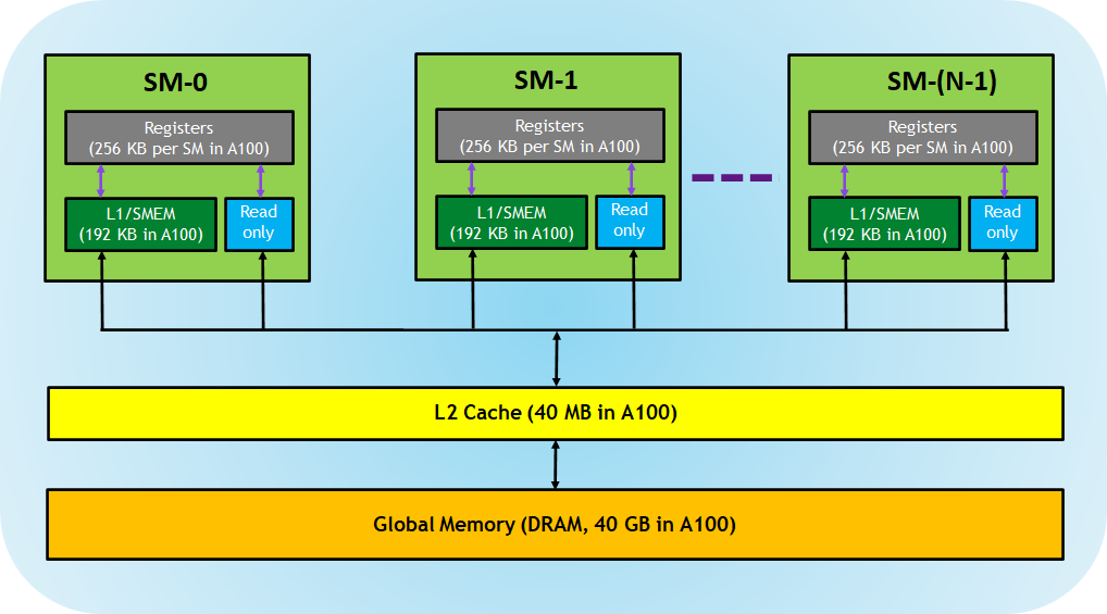
The data movement patterns are straightforward: input tensors () flow from GMEM → SMEM → RF for computation, while output tensor () flows back through RF → SMEM → GMEM. Each step in this pipeline uses different instructions to maximize throughput.

GMEM → SMEM: cp.async

The Ampere architecture added accelerated support for asynchronous loads from GMEM → SMEM. In PTX, these copies encompass the following instructions:

• cp.async: initializes the copy.
  • the size of the copy can be 4, 8, or 16 bytes, just like standard loads
  • when the copy size is 16 bytes, we have the option to configure the transfer to completely bypass the L1 cache, reducing cache pollution and providing a more direct path from L2 to shared memory
  • we’ll use 16 byte copies
• cp.async.commit: combines all uncommitted cp.async’s together into a group that can be waited on as a single entity
• cp.async.wait_group n / cp.async.wait_all: waits until all commits before the latest n groups are complete
  • For example, with 3 groups in flight, cp.async.wait_group 1 waits until
    only 1 group remains in flight (meaning 2 have completed).
  • cp.async.wait() only waits until the current thread has finished loading. If threads are communicating via shared memory, we’ll still need an appropriately scoped barrier for correct synchronization (__syncwarp() / __syncthreads() / cooperative_group.sync()).

For a more in-depth comparison with traditional loads, you can check out the cp.async vs Traditional Loads.

Code

Here are our wrappers for the PTX functions:

ptx_functions.cuh

__device__ void cp_async_commit() { asm volatile("cp.async.commit_group;"); }
 
template <int ngroups>
__device__ void cp_async_wait() {
    asm volatile("cp.async.wait_group %0;" ::"n"(ngroups));
}
 
template <int size, typename T>
__device__ void cp_async(T *smem_to, T *gmem_from) {
    static_assert(size == 16);
    
    uint32_t smem_ptr = __cvta_generic_to_shared(smem_to);
    // The .cg (cache-global) option bypasses the L1 cache, reducing cache 
    // pollution and providing a more direct path from L2 to shared memory.
    asm volatile("cp.async.cg.shared.global [%0], [%1], %2;"
                 :
                 : "r"(smem_ptr), "l"(gmem_from), "n"(size));
}

The call to __cvta_generic_to_shared() converts a generic 64-bit memory address to a 32-bit SMEM-specific address, which is more performant.

LD/ST Operation

Tensors:
Transfer: GMEM → SMEM using cp.async (16B per thread, bytes warp-wide)

SMEM → GMEM: Vectorized Stores

Unfortunately, the equivalent of cp.async for transfers from SMEM → GMEM, st.async, isn’t supported on Ampere, so we’ll go with the next best option: 16 byte vectorized stores. All we have to do is make sure our pointers point to 16-byte data types, and our pointers are 16-byte aligned (addr % 16 == 0).

reinterpret_cast<uint4*>(GMEM[dst])[0] = reinterpret_cast<uint4*>(SMEM[src])[0];

There are some additional nuances to vectorized operations, but we’ll revisit this later when we want to optimize our memory accesses further.

LD/ST Operation

Tensors:
Transfer: SMEM → GMEM using standard stores (16B per thread, warp-wide)

Warp-Wide Transfers Between GMEM ↔ SMEM

When considering warp-wide transfers, we want to ensure memory coalescing for optimal performance. Since GPU cache lines are 128B and each thread transfers 16 bytes, assigning 8 threads to a single row will access the entire cache line. So, with 32 threads per warp, each warp-wide instruction can transfer a tile of memory.

Here’s what a warp covers in a single iteration:

Within a warp, the mapping from a thread to a (row, column) offset is

row = (tid % 32) / 8;
col = tid % 8;

Copying from SMEM → RF

To transfer the fragments into the RF from SMEM, we could load them by having each thread read the elements they store. While this would work, it would require multiple instructions for each fragment. Fortunately, there’s a more efficient approach: the ldmatrix instruction can load up to 4 fragments at a time. It’s faster than loading the fragments manually using RF[dst] = SMEM[src], but has a different layout. This is especially true if we want to also transpose the elements.

ldmatrix

ldmatrix can load 1, 2, or 4 matrix fragments in a single instruction. Each fragment is handled by a group of 8 threads. Threads 0-7 handle the first fragment, 8-15 handle the second, and so on. Here’s a small table that summarizes this:

Fragment	Threads
1	0-7
2	8-15
3	16-23
4	24-31

Within each octet, threads pass in a pointer to their row in SMEM, and the values get broadcast to the entire warp.

Which Fragments to Load?

ldmatrix.x4 lets us load any arbitrary four fragments. That means we could load contiguous or tiles, or even a random set of non-contiguous fragments. This will have an impact on the assembly generated. We’ll revisit this in more detail in kernel 9, but for now, we’ll choose each instruction to transfer tiles of contiguous elements = tiles of fragments. This is the standard and most optimal layout in most cases.

The addressing pattern for ldmatrix differs from the mma fragment layout because it’s optimized for efficient shared memory access patterns. For ldmatrix operations, threads within a warp map to SMEM addresses using:

// ldmatrix addressing (for loading from SMEM to RF)
row = tid % 16;
col = ((tid % 32) / 16) * 8;

which is different from the mappings we saw earlier for mma fragment storage:

// mma fragment storage (for elements within a single fragment)
row = (tid % 32) / 4;  
col = (tid % 4) * 2;

and warp-wide GMEM ↔ SMEM transfer:

row = (tid % 32) / 8;
col = tid % 8;

Here is our wrapper around the PTX function. We also pass in the thread fragment values as uint32_t:

ptx_functions.cuh

template <typename T>
__device__ void ldmatrix_x4(T *load_from, uint32_t &a1, uint32_t &a2,
                            uint32_t &a3, uint32_t &a4) {
    uint32_t smem_ptr = __cvta_generic_to_shared(load_from);
    asm volatile("ldmatrix.sync.aligned.x4.m8n8.shared.b16"
                 "{%0, %1, %2, %3}, [%4];"
                 : "=r"(a1), "=r"(a2), "=r"(a3), "=r"(a4)
                 : "r"(smem_ptr));
}

LD/ST Operation

Tensors:
Transfer: SMEM → RF using ldmatrix.x4, elements = fragments per instruction

ldmatrix Transpose

The ldmatrix instruction has a transpose variant that is the same as ldmatrix except that each fragment is transposed. The transpose occurs only within each fragment, not between fragments. This means that each thread will contain the corresponding values of the transpose:

We use the transposed ldmatrix instruction to load fragments of for computing .

Our wrapper for the transpose version is nearly identical:

ptx_functions.cuh

template <typename T>
__device__ void ldmatrix_x4_transpose(T *load_from, uint32_t &a1, uint32_t &a2,
                                      uint32_t &a3, uint32_t &a4) {
    uint32_t smem_ptr = __cvta_generic_to_shared(load_from);
    asm volatile("ldmatrix.sync.aligned.x4.trans.m8n8.shared.b16"
                 "{%0, %1, %2, %3}, [%4];"
                 : "=r"(a1), "=r"(a2), "=r"(a3), "=r"(a4)
                 : "r"(smem_ptr));
}

To handle the transpose requirement for , we’ll make two changes:

1. We’ll call the transpose variant of ldmatrix to transpose within each fragment
2. We’ll swap the a2 and a3 arguments to transpose between fragments in our tile

Combined, these transpose the entire tile to give us the column-major layout we need for the multiplication. Remember, this is necessary because mma computes , but we want to compute (without the transpose). By storing as effectively in registers, the mma instruction gives us exactly what we need.

LD/ST Operation

Tensors:
Transfer: SMEM → RF using ldmatrix.x4.trans, elements = fragments per instruction

Copying from RF → SMEM

There is an instruction similar to ldmatrix called stmatrix that copies fragments from RF to SMEM. Unfortunately, it’s only available on Hopper and later architectures, so we’ll have to stick with normal 4B SMEM[i] = RF[i]; stores.

The thread to address mapping will follow the mma layout format.

• Inside a fragment, we have 8 rows with 4 threads each.
• Each thread stores 2 values / 4B
• So we can store a single fragment per instruction

LD/ST Operation

Tensors:
Transfer: RF → SMEM using standard stores ( elements = fragment per instruction)

Memory Operations Summary:
We now have efficient pathways for moving data through the memory hierarchy: cp.async for asynchronous GMEM→SMEM transfers, ldmatrix for optimized SMEM→RF loading (with transpose support for ), and standard 4B and 16B stores for the return paths, RF→SMEM and SMEM→GMEM respectively.

Converting Between Data Types

We’ve covered the core matrix operations and memory transfers, but there’s one last piece of the puzzle: data type conversions.

Our mma instruction outputs FP32 values, but we need to convert these to 16-bit precision in two key places:

Softmax output conversion: After computing attention scores and applying softmax (done in FP32 for numerical stability), we need to convert the attention matrix back to 16-bit for the subsequent multiplication. This conversion happens once per iteration.

Final output conversion: The accumulated output vectors stay in FP32 during computation but must be converted to 16-bit before writing back to global memory.

Efficient Paired Conversions

While CUDA provides single-value conversion functions like __float2bfloat16_rn() and __float2half_rn(), we can do better. Since our fragments always contain an even number of values, we can convert two values simultaneously:

• BF16: __float22bfloat162_rn() converts a float2 to bfloat162
• FP16: __float22half2_rn() converts a float2 to half2

This paired approach is more eff.icient because the underlying SASS instructions only support paired conversions. Even single-value conversions get compiled to the paired version with the unused slot filled with zero.

Summary

We’ve covered the essential building blocks for our Flash Attention kernel. Here’s a summary:

The entire pipeline centers around fragments, which are tiles that let threads collaborate efficiently. Each thread stores just 2 elements per fragment, but the mma instruction orchestrates the entire warp to perform matrix multiplication at tensor core speeds.

The memory operations create a careful dance: cp.async streams data from global memory to shared memory asynchronously, ldmatrix efficiently packs fragments into registers, and vectorized stores push results back out. Each step is optimized for Ampere’s specific capabilities. The warp-wide thread to (row, col) mapping formulas are

Operation	Row	Column
mma fragment / RF → SMEM	(tid % 32) / 4	(tid % 4) * 2
SMEM → RF (ldmatrix)	tid % 16	((tid % 32) / 16) * 8
GMEM ↔ SMEM	(tid % 32) / 8	tid % 8

The mma instruction performs the operation D = AB^T + C. The table below specifies the data types and shapes of the operands of the specific variant we’re going to use (m16n8k16).

Operand	DType	Shape (Variables)	Shape (Elements)	Shape (Fragments)	Shape (Registers)
A	BF16/FP16	(m, k)	(16, 16)	(2, 2)	(2, 2)
B	BF16/FP16	(n, k)	(8, 16)	(1, 2)	(1, 2)
C+D	FP32	(m, n)	(16, 8)	(2, 1)	(2, 2)

The load and store operations we perform:

From	To	Blocks	PTX Instr. / C++	Warp-Wide Op Size	Thr. Op Size	Thr. ID Mapping Order	Register Shape	Notes
GMEM	SMEM		cp.async			Row-major
SMEM	RF		ldmatrix.x4			Column-major		transpose
RF	SMEM		standard (4B)			Row-major
SMEM	GMEM		standard (16B)			Row-major

Up Next

With our toolkit of high-performance CUDA operations complete, we’re ready to assemble these pieces into a working Flash Attention kernel. In the next part, we’ll tackle the challenging task of composing these building blocks into a complete implementation. By the end, we’ll have a working Flash Attention kernel achieving around 49% of reference performance.

Footnotes

1. We’ll change this to a 1D array accessed with static strides in kernel 8. ↩